2.2 RBS for depletion scenarios

The ICES-WGFBIT tutorial uses a for-loop to estimate RBS by looping over the RBS-function for each individual grid cell with three inputs: intercept and slope of the binomial longevity model and total depletion. This tutorial splits the RBS-function into two steps.

Create spatrasters of recovery rates

First we create two spatrasters, one for carrying capacity K and one for recovery rates r. Recovery rates are the reciprocal of an arbitrary number of discretized longevity classes L (r=5.31/L). Each discretized longevity class is represented by a layer in the recovery spatraster (rrate_r). Recovery rates of short-lived taxa are higher (e.g. r = 5.31/1 for taxa with a life span of one year) than that of long-lived ones (e.g. r = 5.31/3 for a three year life span). Each longevity class has its specific carrying capacity K, which can be estimated by the area under the curve, or the first derivative of the logistic binomial longevity distribution model using the slope and intercept as described in the ICES-WGFBIT tutorial. Here we create a Spatraster (K_r) for the carrying capacity of each longevity class.

## recovery rates as Spatraster ----
H=5.31 # Hiddink et al 2018 - JAE
size_of_longevity_classes=0.5
longevity=seq(1,200,by=size_of_longevity_classes)
r_template_xy <- terra::xyFromCell(recov_r,1:ncell(recov_r))
long_mt <- cbind(r_template_xy, matrix(rep(longevity,nrow(r_template_xy)),ncol=length(longevity), byrow=T))
colnames(long_mt) <- c("x","y",paste0("longcl_",longevity))
long_r <- terra::rast(long_mt, type="xyz", crs="EPSG:4326")
rrate_r <- H/long_r 
names(rrate_r) <- paste0("r_longcl",longevity)
K_r <- (recov_r[["slope"]]*exp(recov_r[["slope"]]*log(long_r)+recov_r[["intercept"]]))/(long_r * (exp(recov_r[["slope"]]*log(long_r) + recov_r[["intercept"]]) + 1)^2) # 1st derivative of logistic
names(K_r) <- paste0("K_longcl",longevity)

RBS for each of the depletion scenarios

RBS is estimated for each individual grid cell by combining the recovery rates and carrycing capacity of each longevity class with the total depletion caused by the simulated scenarios. Raster algebra allows to estimate the reduction in biomass of each individual longevity class by reducing its carrying capacity with the ratio of depletion over recovery rates of that specific longevity class: \[ \text{B} = K (1 - \frac{d \cdot \text{SAR}}{r}) \] The total biomass after depletion is estimated by grid cell for each of the simulated scenarios by summing the biomass of individual longevity classes, and restraining RBS values between zero and one. The final spatraster rbs_r has multiple layers with RBS values for each of the simulated (mixed fisheries) scenarios (see1.2 Depletion of mixed fisheries scenarios).

## Selection depletion scenarios ----
selnames <- names(deplscen_r)[grep("noCC_Status\\-quo_2021|noCC_FMSY-Min_\\(2025,2030]",names(deplscen_r))]

## RBS estimation of total depletion for selected depletion scenarios ----
rbs_r <- pblapply(deplscen_r[[selnames]], function(rx2){
  temp_r <- (K_r * (1-rx2/rrate_r))
  temp_r <- ifel(temp_r<0,0,temp_r)
  temp_r <- app(temp_r, sum, na.rm=T) * size_of_longevity_classes
  temp_r <- ifel(is.na(temp_r),1,temp_r) # all NAs have no fishing, thus RBS=1
  temp_r <- mask(temp_r, recov_r[["medlong"]])
  return(temp_r)})
names(rbs_r) <- names(deplscen_r[[selnames]])
rbs_r <- rast(rbs_r)

setGDALconfig("GDAL_PAM_ENABLED", "FALSE")
writeRaster(rbs_r,file.path("./output/RBS.tif"), overwrite=TRUE)

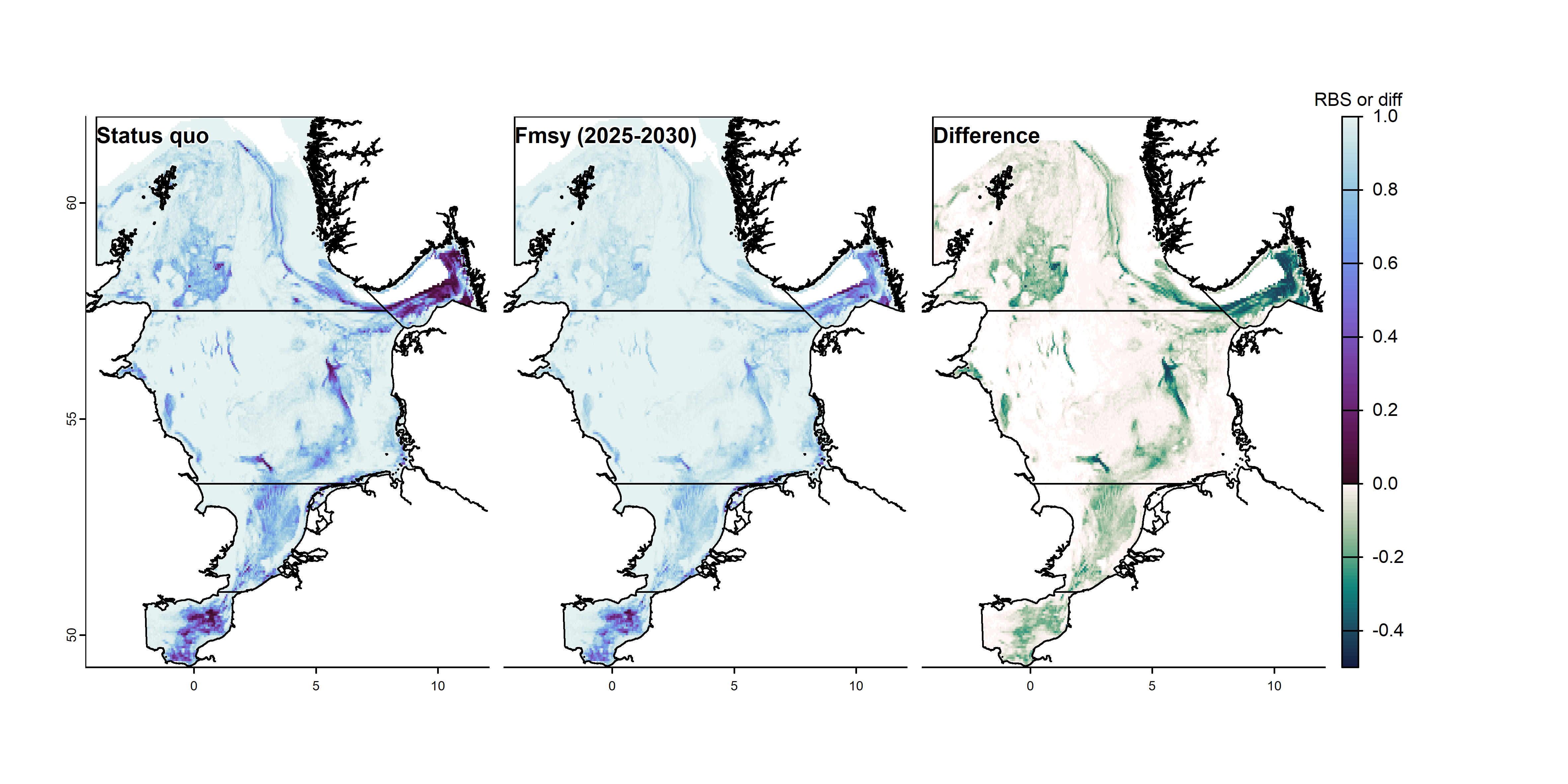
RBS of two mixed fisheries scenarios and their difference